You delegate tasks to a machine rather than doing it yourself so they can do it automatically. You give them precise instructions, and that is your code.
I love Python, particularly pandas’ rich library for data wrangling and mathematical functions.
But today I encountered a limitation of pandas. And it’s predecessor NumPy came through.
I wanted to calculate the average, median, and count of non-null values in a dataset. My dataset is messy and I need to calculate over different columns that aren’t adjacent to each other. For example, I want the average, median and count of all the values in columns 16 and 20. Not 16 through 20. Not the average of column 16, and the average of 20. One single average for the values in both columns 16 and 20.
This is where the “axis” parameter comes in. It usually defaults to axis = 1, ie df.mean(axis = 1), to indicate we are performing the calculation over a single column. For pd.mean(), I used axis = None to get a single mean over two non-adjacent columns. (double-checked it in Excel!)
import pandas as pd
import numpy as np

# df is the dataframe of my full dataset. Here we'll work with a subset of two columns, rows 4 through 54.
hello = df.iloc[4:55, [16, 20]]

# Get mean of the two columns using pandas.mean
calc1 = hello.mean(axis=None)
But pandas doesn’t have an axis = None option for it’s functions to get the median or counts. It only has axis = 0 (over the row) or axis = 1 (over the column) as options, which is inconsistent with the .mean() option.
So this doesn’t work:
calc2 = hello.quantile(0.5, axis=None)
>>> ValueError: No axis named None for object type DataFrame
But hello NumPy! You do have axis=None available for these functions! So let’s import numpy. My dataset has more than half of NaNs (null values) which I didn’t want to include for the median calculation. So I used np.nanquantile() in order not to count them. The np.quantile() function does count them and was returning a median value of ‘NaN’, which wasn’t what I wanted.
For the count function, we are getting a little creative by first counting all of the non-null values in the hello df (using pd.count()), then summing them up so that we can count across all multiple columns.
Thank you NumPy for saving the day! Although pandas is built on NumPy, I’m glad the libraries’ distinct features are all still accessible and that NumPy hasn’t deprecated.
Now that we have a personal SQL database set up in DataGrip, let’s import our first data table. Note that this is for a personal database set up on a local computer. Not a shared database connected to an online server (which is what most companies or organizations would use).
Here’s how to import a table:
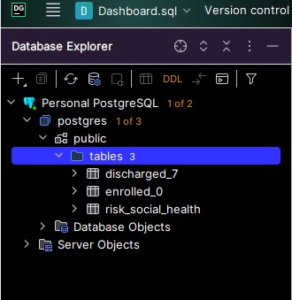
Step 1: Find the “public > tables” folderto which tables will get saved. Starting with a fresh PostgreSQL database set up, this was located in postgres > public > tables. If you do not see a “tables” folder, then use “public”. The tables folder will get automatically created upon importing your first table. Do not use “Database Objects” or “Server Objects”.
Step 2: Right click on “public” or “public > tables” folder > Import/Export > Import Data from File(s).
Step 3: Select the data file to be imported as a table, then ‘OK’. Make sure the file is closed. For example, do not have the .xlsx or .csv open in Excel on your computer, or else you will get an error. Note how many rows of data the original file has (will use for validation in step 5).
Step 4: Set import format settings and set up SQL table. Select the file format (top left corner). Check “First row is header” if it applies (this is not checked by default).Z Set the SQL table name (top right). Review the header names (middle right). Double click on each and rename column names to lowercase with underscores replacing spaces in order to avoid using quotes ” to reference column names in SQL queries. You don’t need to redo this step when importing new data into this table in the future (but you can go back and edit). Click “Import”.
Step 5: Validate that all data rows were imported. A popup will appears in the bottom right corner showing how many rows were imported, and if any, how many errors were written. Check #1: The number of rows imported should match what you expect from the original data file. For example, my data has 64 rows in the original CSV – (1) header row, and (63) data rows. So I expect 63 rows to be imported to the table. If there were any errors, they were not imported into the data table. Investigate, fix, and re-import.
Step 6: Verify that the data looks right. The newly imported table now appears under the “tables” folder on the top left corner. Double click on this to view the table within DataGrip. Check that the data looks correct and as you expect. Issues might include: – Dates are blank or missing values (check that they have the right data type in Step 4, ie Date or Text) – Too many rows: Old data on the table was not deleted, and newly imported data was appended on instead of replacing the old data
I was reading Choose FI: Your Blueprint to Financial Independence and one of the chapters concluded with a question like: “What would you do if you didn’t have to work?”
Something rose to the surface. Even if I didn’t need to work to earn money, I would still practice data analysis using SQL.
This awakened my desire to set up a SQL server-database for personal use. Back-end database access where I can write queries. I miss this dearly from my previous job, where I had an in-house electronic record system and superuser access. I’ve tasted the forbidden fruit and cannot go back to measly front-end, web-browser button clicking to configure reports with limited functionality and flexibility. The power of back-end querying is what I seek, but this is challenging when my company doesn’t currently have a database. Setting one up is notoriously hard, even for professional developers.
I emerged through some struggles to set up a personal SQL database so I can practice queries with my own data. I like the IDE called Datagrip by Jetbrains (free with a student email address) and PostgreSQL (also free) which is what I used in the previous job. Here’s how to set it up.
Step 5: Set up the database in DataGrip. In the “Database” pane on top left, click the + icon > new Data Source > PostgreSQL.
Give it a name. I called it Personal Postgres.
Use localhost, port 5432, and Authentication type as User & Password. Enter the User: Postgres and the Password you defined in step 2. Choose your Save password preference (Forever is convenient for a personal computer).
Test the connection. If it works, then hit Apply and OK.
Note: If you get an error message like this, that means the PostgreSQL was not installed correctly (step 2). You MUST use the username and password. The “No Auth” feature did not work for me.
Step 6: Savor the connection! The database will take a few minutes to connect to an online server so that you can use PostgreSQL SQL functions. If you have very strict firewall settings on your computer, you might need to allow Windows firewall or similar to allow the 5432 port connection.
If everything is good, you’ll get a small Connected status update on the bottom right Event Log:
In a future post, I’ll share how to upload your first database table from a CSV file.
It’s been one year since I started studying programming using Codecademy.com. I set out to study 4 to 5 times a week, every week, 1 lesson page at a time. My longest streak on record is 12 weeks in a row. I’ve completed 86% of the Learn Python 3 course (a hefty course that covers programming fundamentals) and finished the Command Line course too (Linux terminal is not so scary anymore!)
I just finished an online project called ‘Fending the Hacker’ where I read and write to CSV and JSON files programmatically with Python. I didn’t realize this till the end, but this project built on prior lesson topics:
Functions
Loops
Lists
Dictionaries
Modules (JSON, CSV)
Files – Programmatic File Reading/Writing
Looking back on what I’m comfortable with now and how much I’ve learned in one year amazes me. I don’t look back much nor often. But I recall a sinking, confused feeling about not understanding loops, when to use a function, and the purpose of lists and dictionaries. Now I can’t imagine doing any Python analysis or mini project without loops and lists at a minimum. I’m comfortable using them, something distinctly different from before.
This shows me the power of bite-sized but consistent practice. Most lesson topics are divided into about a dozen pages, and I do the reading and practice for 1-2 lesson pages each sitting. That’s 10 minutes or less of light and easy studying. I don’t let long stretches of days pass between each sitting. Recently I’ve shifted my Python study time to earlier in the day to ensure I get it done. I feel the power of compounding knowledge and love it. Is this what the power of compounding interest is also like? The journey along the way has actually been fun.
Onward to the next and final lesson of Python 3, Classes!
The previous post on falsiness (which should be “falseness”, but will continue with the ‘i’ since “Truthiness” is the conceptual term instead of “Truthfulness) has me thinking and steam’s coming out of the engine. I wanted to see for myself these different flavors of False in action, as well as variants of Truthiness.
See the results for yourself running this code in a Python IDE. Experimenting with this made me discover {} is part of the falsiness group, too.
# Values for test: False, 0, None, [], {}

test = []

if test:
    print("True. Condition passed. If statement succeeded.")
else: print("False. Condition did not pass. If statement failed.")
>>> False. Condition did not pass. If statement failed.

test = [1]

if test:
    print("True. Condition passed. If statement succeeded.")
else: print("False. Condition did not pass. If statement failed.")
>>> True. Condition passed. If statement succeeded.
I’ve been coding! Like the slow erosion of a river forming a canyon, I am steadily pecking away at Python to become a better programmer. Here is a lil project I did today. Why chickens? I’ll explain in a future post. Stay tuned! Bok bok bok!
# Magic 8 Ball - Ask a question, reveal an answer.

import random

name = "Heeju"

question = "Should I get hens this weekend?"

answer = ""
answer_2 = ""

# First question random answer generation
random_number = random.randint(1,10)

if random_number == 1:
  answer = "Yes - definitely."
elif random_number == 2:
  answer = "It is decidedly so."
elif random_number == 3:
  answer = "Without a doubt."
elif random_number == 4:
  answer = "Reply hazy, try again."
elif random_number == 5:
  answer = "Ask again later."
elif random_number == 6:
  answer = "Better not to tell you now."
elif random_number == 7:
  answer = "My sources say no."
elif random_number == 8:
  answer = "Outlook not so good."
elif random_number == 9:
  answer = "Very doubtful."
elif random_number == 10:
  answer = "Don't rush it. Give it some time."
else:
  answer = "Error (number outside of range)"

# Second question random answer generation

random_number_2 = random.randint(1,9)
if random_number_2 == 1:
  answer_2 = "Yes - definitely."
elif random_number_2 == 2:
  answer_2 = "It is decidedly so."
elif random_number_2 == 3:
  answer_2 = "Without a doubt."
elif random_number_2 == 4:
  answer_2 = "Reply hazy, try again."
elif random_number_2 == 5:
  answer_2 = "Ask again later."
elif random_number_2 == 6:
  answer_2 = "Better not to tell you now."
elif random_number_2 == 7:
  answer_2 = "My sources say no."
elif random_number_2 == 8:
  answer_2 = "Outlook not so good."
elif random_number_2 == 9:
  answer_2 = "Very doubtful."
else:
  answer_2 = "Error (number outside of range)"


if question == "":
  print("You didn't ask a question. Please ask one!")
elif name == "":
  print(question)
elif name != "":
  print(name,"asks:", question)
else:
  print(name,"asks:", question)


print("Magic 8-ball's answer:", answer)

print("Is this truly random?", answer_2)
As part of my Python programming practice, I came up with a module and function that randomly generates 5 USDA Plant Hardiness Zones / Garden Zones.
def randomgardenzone():
    test_list = ['a', 'b']
    for i in range(1, 5+1):
        x = randint(1, 13)
        res = choice(test_list)
        print(x, res)

randomgardenzone()
For context: the US Department of Agriculture has 13 designated “zones” for the country, based on the average annual min temperature. Each zone number is 10 degrees F apart. There is a further subdivision of zones with a letter ‘a’ or ‘b’, where ‘b’ is 5 degrees F warmer than ‘a’.
These zones are useful for gardeners because we can confidently plant specimens that are hardy (cold/frost/freezing temperature tolerant) to their zone. This is why mango and bananas don’t grow in Minnesota, while they may thrive in a Floridian garden. The Minnesotan would have to have a toasty heated greenhouse in order to cultivate mango trees or bananas through their winter. (Did you know the banana plant is actually an herb, not a tree?)
I’m curious how some plants are able to be cold-hardy and resist freezing. When it gets below 32’F, the water in the plant cells wants to freeze and expand. This would rupture the cell walls and make the plant loose its structure, becoming frost damaged, mushy, and sadly, not salvageable. I heard that cold-hardy plants contain a natural antifreeze that prevents this. I’m curious how antifreeze works, and if it’s similar to what’s used in automobiles. Dianthus is an example of a common plant that is cold-hardy (you can grow them in Alaska), and in fact they need a cold season in order to thrive.
Python Things I learned:
Use “for i in range(1, 5)”, not just “for i in (1,5)”. A simple doh!-type mistake!
range(a, b) works like [a, b) – it is exclusive of the b value. However, randint(a, b) is inclusive of the b value.
The “choice( )” function from the random module let’s you pick a random item from a list. This was useful to pick the zone letters ‘a’ or ‘b’, since randint( ) is only used to pick a random integer.
That’s right, eruptions, not interruptions. We’re talking volcanoes here.
This week’s TidyTuesday theme for R Programming data analysis was on volcanoes, and volcanic eruptions. Data was provided by the Smithsonian Institute.
Did you know all known volcanoes in the world have an official “Volcano Number”?
Did you know that not all volcanic eruptions are confirmed?
For example, since 2000 there have been 794 recorded eruptions, but of these 79 are unconfirmed (about 10%). That’s pretty surprising considering these recently occurred. Perhaps they occurred in very remote regions (like on an unpopulated island in the middle of the Pacific Ocean), or there was dispute if some volcanic activity was considered an “eruption” or not.
Which do you think are the top three countries with confirmed volcanic eruptions since 2000?
Japan came to my mind, but I wasn’t sure about the rest. Maybe Chile or Argentina…
…it turns out, Indonesia (30), Japan (15), USA (14) have had the most confirmed eruptions recently!
The top recent “eruptors” bear very interesting names, like:
Some of these have erupted 22 times in the past 20 years!
You can check out my volcano github post to see more curiosities I analyzed and the actual R programming code I used. I got to learn & practice using some new functions from the dplyr package like:
inner_join(), which combines columns from both datasets in the result semi_join(), which shows only columns from the first specified dataset anti_join(), which keeps only the first dataset’s columns like in semi_join() but feels more rebellious to use
I found this dplyr site helpful in helping me figure out how to use these functions and see which ones fit my analysis needs.
At first, I was bummed that the topic was on “Volcanoes” after a fun whirl on Animal Crossing. However, this analysis turned out to be fun and the time quickly erupted by!